Wave equation
Problem Setup
The general solution is given by: \(u(x,t) = F(x-ct) + G(x+ct)\) with F, G some functions.
Take \(F(x) = x^2\) and \(G(x) = \sin(x)\) and \(c=1\).
Thus: \(u(x,t) = (x-t)^2 + \sin(x + t)\).
Set \(f = 0\).
Consider \(u\) to be a Gaussian process:
\(u \sim \mathcal{GP}(0, k_{uu}(x_i, x_j; \tilde{\theta}))\) with the hyperparameters \(\tilde{\theta} = \{\theta, l_x, l_t\}\).
And the linear operator:
\(\mathcal{L}_x^c = \frac{d^2}{dt^2} \cdot - c \frac{d^2}{dx^2} \cdot\)
so that
\(\mathcal{L}_x^c u = f\)
Problem at hand: Estimate \(c\) (should be \(c = 1\) in the end).
Step 1: Simulate data
\(x \in [0, 1]^n, \; t \in [0,1]^n\)
In [3]:
def get_simulated_data(n = 20):
    t = np.random.rand(n)
    x = np.random.rand(n)
    y_u = np.multiply(x-t, x-t) + np.sin(x+t)
    y_f = 0*x
    return(x, t, y_u, y_f)

(x, t, y_u, y_f) = get_simulated_data()
Step 2: Evaluate kernels
- \(k_{uu}(y_i, y_j; \tilde{\theta}) = \theta exp(-\frac{1}{2l_x}(x_i-x_j)^2 - \frac{1}{2l_t}(t_i-t_j)^2)\), where \(y_i = (x_i, t_i)\), \(y_j = (x_j, t_j)\).
- \(k_{ff}(y_i,y_j; \tilde{\theta}, c) = \mathcal{L}_{y_i}^c \mathcal{L}_{y_j}^c k_{uu}(y_i, y_j; \tilde{\theta}) \\ = \frac{d^4}{dt_i^2 dt_j^2}k_{uu} - c\frac{d^4}{dt_i^2 dx_j^2}k_{uu} - c\frac{d^4}{dx_i^2 dt_j^2}k_{uu} + c^2\frac{d^4}{dx_i^2 dx_j^2}k_{uu}\)
- \(k_{fu}(y_i,y_j;\tilde{\theta}, c) = \mathcal{L}_{\tilde{x}_i}^c k_{uu}(y_i, y_j; \tilde{\theta}) = \frac{d^2}{dt_i^2}k_{uu} - c\frac{d^2}{dx_i^2}k_{uu}\)
- \(k_{uf}(y_i, y_j; \tilde{\theta}, c)\) is given by the transpose of \(k_{fu}(y_i, y_j; \tilde{\theta}, c)\).
Steps 3 and 4: Compute NLML and optimize the hyperparameters
In [10]:
m = minimize_restarts(x, t, y_u, y_f, 5)
np.exp(m.x[3]) # This is the optimized value for our parameter c
Out[10]:
0.9978007101765757
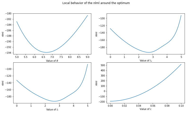
Step 5: Plotting the behavior for varied parameters
The logarithms of the optimal hyperparameters are given by (arranged in \([\theta, l_x, l_t, c]\)):
In [11]:
m.x
Out[11]:
array([ 6.67851868e+00, 2.71167786e+00, 2.66415024e+00, -2.20171181e-03])
We want to plot the behavior of the nlml-function around the minimizer:
In [13]:
show_1(lin0, lin1, lin3, res0, res1, res2, res3);
Step 6: Analysis of the error
In this section we want to analyze the error of our algorithm using two different ways and plot its time complexity.
1. Plotting the error in our estimate for c:
The error is given by \(| c_{estimate} - c_{true} |\).
We ran the algorithm five times and plotted the respective outcomes in different colors:
In [33]:
show_3(lin, ones, res)
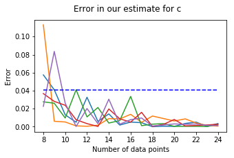
We see that for n sufficiently large (in this case \(n \geq 10\)), we can assume the error to be bounded by 0.041.
2. Plotting the error between the solution and the approximative solution:
In [39]:
show_4(lin, ones, res, diff)
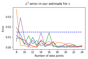
The \(L^2\)-error is in our case bounded by 0.015 for \(n \geq 10\).
3. Plotting the execution time:
In [42]:
show_5(lin, timing)
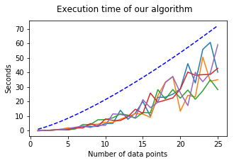
Curiously, the time complexity seems to be around \(\mathcal{O}(n^{4/3})\) (blue-dashed line).
Assuming an equal amount of function evaluations in the Nelder-Mead algorithm for different values of n, we would have been expecting a time complexity of \(\mathcal{O}(n^3)\), due to the computation of the inverse of an \(n\times n\)-matrix in every evaluation of \(\textit{nlml}\). This could probably be seen with larger values of n.