Heat equation

The heat equation is a parabolic partial differential equation that describes the distribution of heat (or variation in temperature) in a given region over time. The general form of the equation in any coordinate system is given by:

:raw-latex:`\begin{align*} \frac{\partial u}{\partial t} - \phi \nabla^2 u = f \end{align*}`

We will work here with the heat equation in one spatial dimension. This can be formulated as:

:raw-latex:`\begin{align*} \mathcal{L}_{\bar{x}}^{\phi}u(\bar{x}) = \frac{\partial}{\partial t}u(\bar{x}) - \phi \frac{\partial^2}{\partial x^2}u(\bar{x}) = f(\bar{x}), \end{align*}` where \(\bar{x} = (t, x) \in \mathbb{R}^2\).

The fundamental solution to the heat equation gives us:

:raw-latex:`\begin{align*} u(x,t) &= e^{-t}sin(2\pi x) \\ f(x,t) &= e^{-t}(4\pi^2 - 1)sin(2\pi x) \end{align*}`

Simulate data

np.random.seed(int(time.time()))
def get_simulated_data(n):
    t = np.random.rand(n)
    x = np.random.rand(n)
    y_u = np.multiply(np.exp(-t), np.sin(2*np.pi*x))
    y_f = (4*np.pi**2 - 1) * np.multiply(np.exp(-t), np.sin(2*np.pi*x))
    return (t, x, y_u, y_f)

(t, x, y_u, y_f) = get_simulated_data(10)

Evaluate kernels

We use a reduced version of the kernel here.

1. \(k_{uu}(x_i, x_j, t_i, t_j; \theta) = e^ \left[ -\theta_1 (x_i-x_j)^2 - \theta_2 (t_i-t_j)^2 \right]\)
2. \(k_{ff}(\bar{x}_i,\bar{x}_j;\theta,\phi) = \mathcal{L}_{\bar{x}_i}^\phi \mathcal{L}_{\bar{x}_j}^\phi k_{uu}(\bar{x}_i, \bar{x}_j; \theta) = \mathcal{L}_{\bar{x}_i}^\phi \left[ \frac{\partial}{\partial t_j}k_{uu} - \phi \frac{\partial^2}{\partial x_j^2} k_{uu} \right] \\ = \frac{\partial}{\partial t_i}\frac{\partial}{\partial t_j}k_{uu} - \phi \left[ \frac{\partial}{\partial t_i}\frac{\partial^2}{\partial x_j^2}k_{uu} + \frac{\partial^2}{\partial x_i^2}\frac{\partial}{\partial t_j}k_{uu} \right] + \phi^2 \frac{\partial^2}{\partial x_i^2}\frac{\partial^2}{\partial x_j^2}k_{uu}\)
3. \(k_{fu}(\bar{x}_i,\bar{x}_j;\theta,\phi) = \mathcal{L}_{\bar{x}_i}^\phi k_{uu}(\bar{x}_i, \bar{x}_j; \theta) = \frac{\partial}{\partial t_i}k_{uu} - \phi \frac{\partial^2}{\partial x_i^2}k_{uu}\)

Optimize hyperparameters

%%timeit
nlml_wp = lambda params: nlml(params, t, x, y_u, y_f, 1e-7)
minimize(
    nlml_wp,
    np.random.rand(3),
    method="Nelder-Mead",
    options={'maxiter' : 5000, 'fatol' : 0.001})

2.13 s ± 267 ms per loop (mean ± std. dev. of 7 runs, 1 loop each)

def minimize_restarts(t, x, y_u, y_f, n = 10):
    nlml_wp = lambda params: nlml(params, t, x, y_u, y_f, 1e-7)
    all_results = []
    for it in range(0,n):
        all_results.append(
            minimize(
                nlml_wp,
                np.random.rand(3),
                method="Nelder-Mead",
                options={'maxiter' : 5000, 'fatol' : 0.001}))
    filtered_results = [m for m in all_results if 0 == m.status]
    return min(filtered_results, key = lambda x: x.fun)

Estimated value of \(\alpha\)

np.exp(m.x[2])

0.9701718328188159

Analysis

Contour lines for the likelihood

plt.show()

Profile likelihood

plt.show()

Errors

We generate 5 set of samples for each number of data points(n) in the range (5,25) as earlier. The absolute error in the parameter estimate and the computation times are plotted in the following figure.

plt.show()

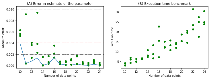
The minimum error for each value of n is bounded by 0.002 for n > 10. The computation time also increases monotonically with n.

With the full kernel

nlml((1,1,1,0), t, x, y_u, y_f, 1e-6)

1100767.8910308597

%%timeit
nlml_wp = lambda params: nlml(params, t, x, y_u, y_f, 1e-7)
minimize(
    nlml_wp,
    np.random.rand(4),
    method="Nelder-Mead",
    options={'maxiter' : 5000, 'fatol' : 0.001})

6.93 s ± 1.94 s per loop (mean ± std. dev. of 7 runs, 1 loop each)

The reduced kernel takes less time for optimization as compared to the full one.

plt.show()

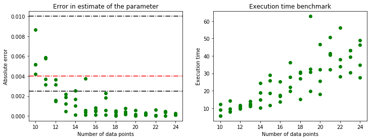
The same analysis as earlier in the chapter was done for the full kernel given by \(\theta exp((\mathbf{x}-\mathbf{y})^T \Sigma (\mathbf{x}-\mathbf{y}))\) where \(\Sigma = diag([l_1, l_2])\).

It can be noticed that the error in parameter estimate is slightly lower for the full kernel but the difference is not very significant. Meanwhile, the execution times are significantly different for both the cases. For 10 data points, the minimizer takes an average of 2.13 seconds for the reduced kernel while it is 6.93 seconds for the full kernel. This shows that not all hyperparameters might be necessary to get acceptable results. For some specific problems, having an intuition on the choice of kernels might be fruitful in the end.