The inviscid Burgers’ Equation

Problem Setup

Then \(u_0(x) := u(x,0) = x\)

Using the backward Euler scheme, the equation can be re-written as:

We set \(u_n = \mu_{n-1}\), where \(\mu_{n-1}\) is the mean of \(u_{n-1}\), to deal with the non-linearity:

Consider \(u_n\) to be a Gaussian process.

\(u_n \sim \mathcal{GP}(0, k_{uu}(x_i, x_j; \theta, l))\)

And the linear operator:

\(\mathcal{L}_x^c = \cdot + \tau c \mu_{n-1} \frac{d}{dx}\cdot\)

so that

\(\mathcal{L}_x^c u_n = u_{n-1}\)

Problem at hand: Estimate \(c\). Using 20 data points, we will be able to estimate c to be 0.9994.

For the sake of simplicity, take \(u := u_n\) and \(f := u_{n-1}\).

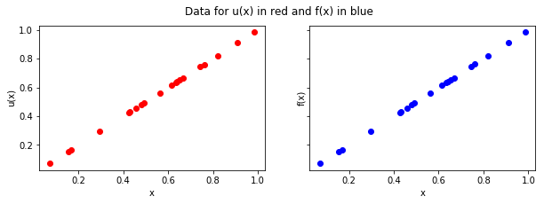
Step 1: Simulate data

Take data points at \(t = 0\) for \((u_{n-1})\) and \(t = \tau\) for \((u_n)\), where \(\tau\) is the time step.

\(x \in [0, 1], \; t \in \{0, \tau \}\)

tau = 0.001
def get_simulated_data(tau, n=20):
    x = np.random.rand(n)
    y_u = x/(1+tau)
    y_f = x
    return (x, y_u, y_f)

(x, y_u, y_f) = get_simulated_data(tau)

show_1(x,y_u,y_f)

Step 2: Evaluate kernels

1. \(k_{uu}(x_i, x_j; \theta, l) = \theta exp(-\frac{1}{2l}(x_i-x_j)^2)\), where \(\theta, l > 0\)
2. \(k_{ff}(x_i,x_j;\theta, l, c) = \mathcal{L}_{x_i}^c \mathcal{L}_{x_j}^c k_{uu}(x_i, x_j; \theta, l) \\ = k_{uu} + \tau c \mu_{n-1} \frac{d}{dx_i}k_{uu} + \tau c \mu_{n-1} \frac{d}{dx_j}k_{uu} + \tau^2 c^2 \mu_{n-1}^2 \frac{d^2}{d x_i x_j} k_{uu}\)
3. \(k_{fu}(x_i,x_j; \theta, l, c) = \mathcal{L}_{x_i}^c k_{uu}(x_i, x_j; \theta, l) \\ = k_{uu} + \tau \mu_{n-1} c \frac{d}{dx_i}k_{uu}\)
4. \(k_{uf}(x_i,x_j;\theta, l, c)\) is given by the transpose of \(k_{fu}(x_i,x_j;\theta, l, c)\)

Steps 3 and 4: Compute NLML and optimize the hyperparameters

m = minimize(nlml, np.random.rand(3), args=(x, y_u, y_f, 1e-7), method=\
             "Nelder-Mead", options = {'maxiter' : 1000})

m.x[2]  # This is our inferred value for c

0.9994300669651587

Step 5: Analysis w.r.t. the number of data points (up to 25):

In this section we want to analyze the error of our algorithm using two different ways and plot its time complexity.

1. Plotting the error in our estimate for c:

The error is given by \(| c_{estimate} - c_{true} |\).

We have altogether ran the algorithm five times, each time increasing the number of data points:

show_2(lin, ones, res)

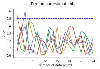
We see that for n sufficiently large (in this case \(n \geq 5\)), we can assume the error to be bounded by 0.5. It seems to be difficult to (even roughly) describe the limiting behavior of the error w.r.t. the number of data points.

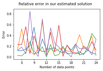
2. Plotting the error between the solution and the approximative solution:

show_2(lin, ones, res)

<Figure size 360x216 with 0 Axes>

3. Plotting the execution time:

All in one plot (the blue dashed line follows \(f(x) = 0.01x^{2.2}\)):

show_3(lin, timing)

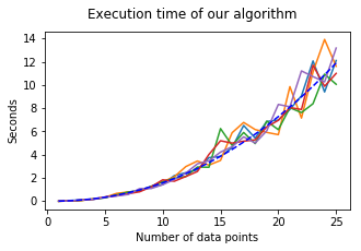
The time complexity seems to be around \(\mathcal{O}(n^{2.2})\) (blue-dashed line).