The inviscid Burgers’ Equation - A different approach

Problem Setup

Setting \(u(x,t) = \frac{x}{1+t}\), we expect \(\nu = 0\) as a parameter.

Then \(u_0(x) := u(x,0) = x\).

Using the forward Euler scheme, the equation can be re-written as:

and setting the factor \(u_{n-1} = \mu_{n-1}\) (analogously to the previous subchapter this is the mean of \(u_{n-1}\)) to deal with the non-linearity:

Consider \(u_{n-1}\) to be a Gaussian process.

\(u_{n-1} \sim \mathcal{GP}(0, k_{uu}(x_i, x_j; \theta, l))\)

And the linear operator:

\(\mathcal{L}_x^\nu = \cdot + \tau \nu \frac{d}{dx}\cdot - \tau \mu_{n-1} \frac{d}{dx} \cdot\)

so that

\(\mathcal{L}_x^\nu u_{n-1} = u_n\)

Problem at hand: Estimate \(\nu\) (should be \(\nu = 0\) in the end).

For the sake of simplicity, take \(u := u_{n-1}\) and \(f := u_n\).

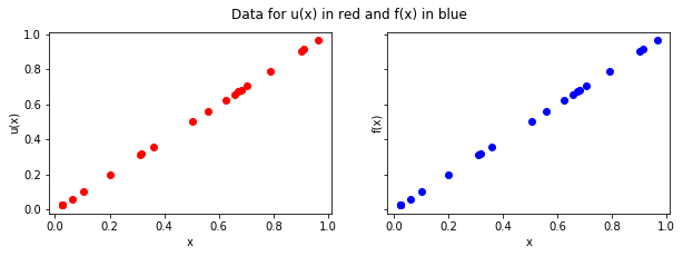
Step 1: Simulate data

Take data points at \(t = 0\) for \((u_{n-1})\) and \(t = \tau\) for \((u_n)\), where \(\tau\) is the time step.

\(x \in [0, 1], \; t \in \{0, \tau \}\)

tau = 0.001
def get_simulated_data(tau, n=20):
    x = np.random.rand(n)
    y_u = x
    y_f = x/(1+tau)
    return (x, y_u, y_f)

(x, y_u, y_f) = get_simulated_data(tau)

show_1(x, y_u, y_f)

Step 2: Evaluate kernels

1. \(k_{uu}(x_i, x_j; \theta, l) = \theta exp(-\frac{1}{2l}(x_i-x_j)^2)\)
2. \(k_{ff}(x_i,x_j;\theta, l,\nu) = \mathcal{L}_{x_i}^\nu \mathcal{L}_{x_j}^\nu k_{uu}(x_i, x_j; \theta, l) \\ = k_{uu} + \tau \nu \frac{d}{dx_i}k_{uu} - \tau \mu_{n-1} \frac{d}{dx_i}k_{uu} + \tau \nu \frac{d}{dx_j}k_{uu} + \tau^2 \nu^2 \frac{d}{dx_i} \frac{d}{dx_j}k_{uu} - \tau^2 \nu \mu_{n-1}\frac{d^2}{dx_i dx_j} k_{uu} - \tau \mu_{n-1} \frac{d}{dx_j}k_{uu} - \tau^2 \nu \mu_{n-1} \frac{d^2}{dx_i dx_j} k_{uu} + \tau^2 \mu_{n-1}^2 \frac{d^2}{dx_i dx_j}k_{uu}\)
3. \(k_{fu}(x_i,x_j;\theta,l,\nu) = \mathcal{L}_{x_i}^\nu k_{uu}(x_i, x_j; \theta, l) \\ = k_{uu} + \tau \nu \frac{d}{dx_i}k_{uu} - \tau \mu_{n-1}\frac{d}{dx_i}k_{uu}\)
4. \(k_{uf}(x_i,x_j;\theta, l, \nu)\) is given by the transpose of \(k_{fu}(x_i,x_j;\theta, l, \nu)\).

Steps 3 and 4: Compute NLML and optimize the hyperparameters

m = minimize(nlml, np.random.rand(3), args=(x, y_u, y_f, 1e-7), method=\
             "Nelder-Mead", options = {'maxiter' : 1000})

m.x[2]   # This is our inferred value for \nu

0.00021347647791778476

Step 5: Analysis w.r.t. the number of data points (up to 25):

In this section we want to analyze the error of our algorithm and plot its time complexity.

1. Plotting the error in our estimate:

The error is given by \(| \nu_{estimate} - \nu_{true} |\).

We plot the error with respect to the number of data samples for five runs of the program:

show_2(lin, res)

<Figure size 360x216 with 0 Axes>

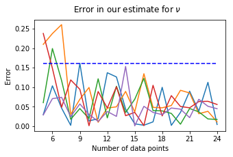
We see that for n sufficiently large (in this case \(n \geq 8\)), we can assume the error to be bounded by 0.16.

2. Plotting the error between the solution and the approximative solution:

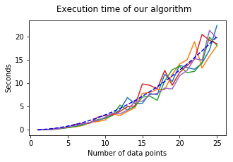
3. Plotting the execution time:

The blue-dashed line follows \(f(x) = 0.032 x^2\).

show_3(lin, timing)

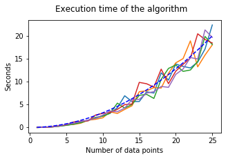
We observe a time complexity of roughly \(\mathcal{O}(n^2)\) (blue-dashed line).

Comparison with a no-mean version

\(\tau \nu \frac{d^2}{dx^2}u_{n-1} - \tau x \frac{d}{dx}u_{n-1} + u_{n-1} = u_{n}\)

The linear operator looks just slightly different:

\(\mathcal{L}_x^\nu = \cdot + \tau \nu \frac{d}{dx}\cdot - \tau x \frac{d}{dx} \cdot\)

so that

\(\mathcal{L}_x^\nu u_{n-1} = u_n\).

Our kernels evaluate to:

1. \(k_{uu}(x_i, x_j; \theta, l) = \theta exp(-\frac{1}{2l}(x_i-x_j)^2)\)
2. \(k_{ff}(x_i,x_j;\theta, l,\nu) = \mathcal{L}_{x_i}^\nu \mathcal{L}_{x_j}^\nu k_{uu}(x_i, x_j; \theta, l) \\ = k_{uu} + \tau \nu \frac{d}{dx_i}k_{uu} - \tau x \frac{d}{dx_i}k_{uu} + \tau \nu \frac{d}{dx_j}k_{uu} + \tau^2 \nu^2 \frac{d}{dx_i} \frac{d}{dx_j}k_{uu} - \tau^2 \nu x\frac{d^2}{dx_i dx_j} k_{uu} - \tau x \frac{d}{dx_j}k_{uu} - \tau^2 \nu x \frac{d^2}{dx_i dx_j} k_{uu} + \tau^2 x^2 \frac{d^2}{dx_i dx_j}k_{uu}\)
3. \(k_{fu}(x_i,x_j;\theta,l,\nu) = \mathcal{L}_{x_i}^\nu k_{uu}(x_i, x_j; \theta, l) \\ = k_{uu} + \tau \nu \frac{d}{dx_i}k_{uu} - \tau x\frac{d}{dx_i}k_{uu}\)
4. \(k_{uf}(x_i,x_j;\theta, l, \nu)\) is given by the transpose of \(k_{fu}(x_i,x_j;\theta, l, \nu)\).

After constructing the nlml we get:

m = minimize(nlml, np.random.rand(3), args=(x, y_u, y_f, 1e-7), method=\
             "Nelder-Mead", options = {'maxiter' : 1000})
m.x[2] # This is our prediction for \nu

0.00042724953581625225

We can analyze the error in multiple runs and look at the execution time:

1. Plotting the error in our estimate for \(\nu\)

The error is given by \(| \nu_{estimate} - \nu_{true} |\).

show_4(lin, est, res)

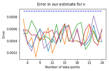
We see that for n sufficiently large (in this case \(n \geq 5\)), we can assume the error to be bounded by 0.0009.

2. Plotting the execution time:

show_5(lin, timing)

The time complexity seems to be as before roughly \(\mathcal{O}(n^2)\).