2D Linear operator with one parameter

Along the same lines as the previous example, we take a two-dimensional linear operator corresponding to a two-dimensional system with a single parameter. As previously explained, we set our problem up as follows:

It is easy to verify that \(\mathcal{L}_\bar{x}^\phi\) is linear and continuous. A suitable solution for the operator is

:raw-latex:`\begin{align*} u(\bar{x}) &= x_1 x_2 - x_2^2 \\ f(\bar{x}) &= \phi x_1 x_2 - \phi x_2^2 + x_2 - 2 \end{align*}`

Now, we use the same Gaussian priors as before, except that they are now defined on a two-dimensional space.

:raw-latex:`\begin{align*} u(\bar{x}) &\sim \mathcal{GP}(0, k_{uu}(\bar{x},\bar{x}',\theta)) \\ f(\bar{x}) &\sim \mathcal{GP}(0, k_{ff}(\bar{x},\bar{x}',\theta,\phi)) \\ y_u &= u(X) + \epsilon_u; \; \epsilon_u \sim \mathcal{N}(0, \sigma_u^2I) \\ y_f &= f(X) + \epsilon_f; \; \epsilon_f \sim \mathcal{N}(0, \sigma_f^2I) \end{align*}`

The parameter estimation problem for the linear operator described above is to estimate \(\phi\), given \(\{x, y_u, y_f\}\). Notice that we evaluate \(u, f\) on the same set of points because it makes sense from a physics point of view.

Simulate data

We use \(\phi = 2\) and try to estimate it.

def get_simulated_data(n, phi):
    x = np.random.rand(n,2)
    y_u = np.multiply(x[:,0], x[:,1]) - x[:,1]**2
    y_f = phi*y_u + x[:,1] - 2
    return (x, y_u, y_f)

Evaluate kernels

The implementation of the kernels is straightforward as done earlier. Consequently, the corresponding code has been omitted from the report.

1. \(k_{uu}(\bar{x}_i, \bar{x}_j; \theta) = \theta e^{(-l_1 (x_{i,1}-x_{j,1})^2 -l_2 (x_{i,2}-x_{j,2})^2)}\)
2. \(k_{ff}(\bar{x}_i,\bar{x}_j;\theta,\phi) = \mathcal{L}_{\bar{x}_i}^\phi \mathcal{L}_{\bar{x}_j}^\phi k_{uu}(\bar{x}_i, \bar{x}_j; \theta) \\ = \mathcal{L}_{\bar{x}_i}^\phi \left( \phi k_{uu} + \frac{\partial}{\partial x_{j,1}}k_{uu} + \frac{\partial^2}{\partial^2 x_{j,2}}k_{uu}\right) \\ = \phi^2 k_{uu} + \phi \frac{\partial}{\partial x_{j,1}}k_{uu} + \phi \frac{\partial}{\partial x_{i,1}}k_{uu} \\ \quad + \phi \frac{\partial^2}{\partial^2 x_{j,2}}k_{uu} + \frac{\partial}{\partial x_{i,1}}\frac{\partial}{\partial x_{j,1}}k_{uu} + \phi \frac{\partial^2}{\partial^2 x_{i,2}}k_{uu} \\ \quad + \frac{\partial}{\partial x_{i,1}}\frac{\partial^2}{\partial^2 x_{j,2}}k_{uu} + \frac{\partial^2}{\partial^2 x_{i,2}}\frac{\partial}{\partial x_{j,1}}k_{uu} + \frac{\partial^2}{\partial^2 x_{i,2}}\frac{\partial^2}{\partial^2 x_{j,2}}k_{uu}\)
3. \(k_{fu}(\bar{x}_i,\bar{x}_j;\theta,\phi) = \mathcal{L}_{\bar{x}_i}^\phi k_{uu}(\bar{x}_i, \bar{x}_j; \theta) \\ = \phi k_{uu} + \frac{\partial}{\partial x_{i,1}}k_{uu} + \frac{\partial^2}{\partial x_{i,2}^2}k_{uu}\)

(x, yu, yf) = get_simulated_data(10, 2)
nlml((1, 1, 1, 0.69), x, yu, yf, 1e-6)

10.124377463652147

Optimize hyperparameters

nlml_wp = lambda params: nlml(params, x, yu, yf, 1e-7)
m = minimize(nlml_wp, np.random.rand(4), method="Nelder-Mead")

np.exp(m.x)

array([1.29150445e+06, 4.54133519e-05, 5.27567407e-04, 2.00497047e+00])

The optimized hyperparameters are:

Parameter	Value
\(\theta\)	1.29150445e+06
\(l_1\)	4.54133519e-05
\(l_2\)	5.27567407e-04
\(\phi\)	2.00497047

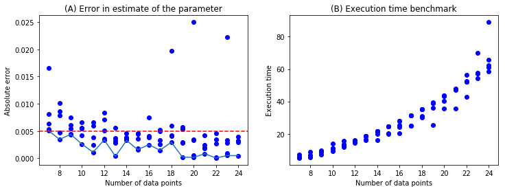
Analysis

To investigate error properties for this model, we run simulations from 5 to 25 datapoints with 5 samples of random data in each case which is 100 samples. The absolute error in the parameter estimate, \(|\phi_{est} - \phi_{true}|\) is plotted in the left figure below. The execution time is plotted to the right; it includes the time taken to simulate the data and the time taken by the optimization routine.

plt.show()