1D Linear operator with one parameter

This chapter introduces a basic example of the framework developed in Chapter 3. We take a one-dimensional system with a single parameter and extract an operator out of it.

:raw-latex:`\begin{align*} \mathcal{L}_x^\phi u(x) &= f(x) \\ \mathcal{L}_x^\phi &:= \phi \cdot + \frac{d}{dx}\cdot \end{align*}`

It is trivial to verify linearity of the operator:

:raw-latex:`\begin{align*} u, f : [0, 1] &\rightarrow \mathbb{K}, \alpha, \beta \in \mathbb{R} \\ \mathcal{L}_x^\phi (\alpha u + \beta f) &= \phi (\alpha u + \beta f) + \frac{d}{dx}(\alpha u + \beta f) \\ &= \alpha \phi u + \beta \phi f + \alpha \frac{d}{dx}u + \beta \frac{d}{dx}f \\ &= \alpha \mathcal{L}_x^\phi u + \beta \mathcal{L}_x^\phi f \end{align*}`

One of the solutions to this system might be:

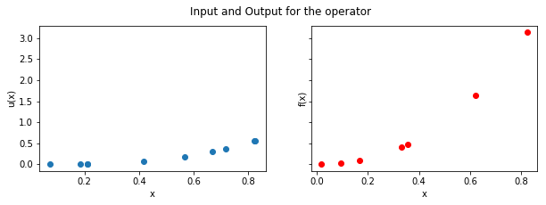
:raw-latex:`\begin{align*} u(x) &= x^3 \\ f(x) &= \phi x^3 + 3x^2 \\ x &\in [0, 1] \end{align*}`

We define Gaussian priors on the input and output:

:raw-latex:`\begin{align*} u(x) &\sim \mathcal{GP}(0, k_{uu}(x,x',\theta)) \\ f(x) &\sim \mathcal{GP}(0, k_{ff}(x,x',\theta,\phi)) \end{align*}`

A noisy data model for the above system can be defined as:

:raw-latex:`\begin{align*} y_u &= u(X_u) + \epsilon_u; \epsilon_u \sim \mathcal{N}(0, \sigma_u^2I)\\ y_f &= f(X_f) + \epsilon_f; \epsilon_f \sim \mathcal{N}(0, \sigma_f^2I) \end{align*}`

For the sake of simplicity, we ignore the noise terms \(\epsilon_u\) and \(\epsilon_f\) while simulating the data. They’re nevertheless beneficial, when computing the negative log marginal likelihood (NLML) so that the resulting covariance matrix is mostly more well-behaved for reasons as they were outlined after the preface.

For the parameter estimation problem for the linear operator described above, we are given \(\{X_u, y_u\}\), \(\{X_f, y_f\}\) and we need to estimate \(\phi\).

Step 1: Simulate data

We use \(\phi = 2\).

def get_simulated_data(n1, n2, phi):
    x_u = np.random.rand(n1)
    y_u = np.power(x_u, 3)
    x_f = np.random.rand(n2)
    y_f = phi*np.power(x_f, 3) + 3*np.power(x_f,2)
    return(x_u, y_u, x_f, y_f)

plt.show()

Step 2: Evaluate kernels

We use the RBF kernel defined as:

:raw-latex:`\begin{align*} k_{uu}(x_i, x_j; \theta) = \theta exp(-\frac{1}{2l}(x_i-x_j)^2) \end{align*}`

throughout the report. It is worth noting that this step uses information about \(\mathcal{L}_x^\phi\) but not about \(u(x)\) or \(f(x)\). The derivatives are computed using sympy.

x_i, x_j, theta, l, phi = sp.symbols('x_i x_j theta l phi')
kuu_sym = theta*sp.exp(-l*((x_i - x_j)**2))
kuu_fn = sp.lambdify((x_i, x_j, theta, l), kuu_sym, "numpy")
def kuu(x, theta, l):
    k = np.zeros((x.size, x.size))
    for i in range(x.size):
        for j in range(x.size):
            k[i,j] = kuu_fn(x[i], x[j], theta, l)
    return k

:raw-latex:`\begin{align*} k_{ff}(x_i,x_j;\theta,\phi) &= \mathcal{L}_{x_i}^\phi \mathcal{L}_{x_j}^\phi k_{uu}(x_i, x_j; \theta) \\ &= \mathcal{L}_{x_i}^\phi \left( \phi k_{uu} + \frac{\partial}{\partial x_j}k_{uu} \right) \\ &= \phi^2 k_{uu} + \phi \frac{\partial}{\partial x_j}k_{uu} + \phi \frac{\partial}{\partial x_i}k_{uu} + \frac{\partial}{\partial x_i}\frac{\partial}{\partial x_j}k_{uu} \\ &= \theta exp(-\frac{1}{2l}(x_i-x_j)^2)\left[ \phi^2 + 2\phi |x_i-x_j| + (x_i-x_j)^2 + 1 \right] \end{align*}`

kff_sym = phi**2*kuu_sym \
            + phi*sp.diff(kuu_sym, x_j) \
            + phi*sp.diff(kuu_sym, x_i) \
            + sp.diff(kuu_sym, x_j, x_i)
kff_fn = sp.lambdify((x_i, x_j, theta, l, phi), kff_sym, "numpy")
def kff(x, theta, l, phi):
    k = np.zeros((x.size, x.size))
    for i in range(x.size):
        for j in range(x.size):
            k[i,j] = kff_fn(x[i], x[j], theta, l, phi)
    return k

:raw-latex:`\begin{align*} k_{fu}(x_i,x_j;\theta,\phi) &= \mathcal{L}_{x_i}^\phi k_{uu}(x_i, x_j; \theta) \\ &= \phi k_{uu} + \frac{\partial}{\partial x_i}k_{uu} \\ &= \theta exp(-\frac{1}{2l}(x_i-x_j)^2) \left[ (\frac{1}{2})2|x_i-x_j| + \phi \right] \\ &= \theta exp(-\frac{1}{2l}(x_i-x_j)^2)(\phi + |x_i-x_j|) \end{align*}`

kfu_sym = phi*kuu_sym + sp.diff(kuu_sym, x_i)
kfu_fn = sp.lambdify((x_i, x_j, theta, l, phi), kfu_sym, "numpy")
def kfu(x1, x2, theta, l, phi):
    k = np.zeros((x2.size, x1.size))
    for i in range(x2.size):
        for j in range(x1.size):
            k[i,j] = kfu_fn(x2[i], x1[j], theta, l, phi)
    return k

:raw-latex:`\begin{align*} k_{uf}(x_i,x_j;\theta,\phi) &= \mathcal{L}_{x_j}^\phi k_{uu}(x_i, x_j; \theta) \\ &= \phi k_{uu} + \frac{\partial}{\partial x_j}k_{uu} \\ &= \theta exp(-\frac{1}{2l}(x_i-x_j)^2) \left[ (\frac{1}{2})2|x_i-x_j| + \phi \right]\\ &= \theta exp(-\frac{1}{2l}(x_i-x_j)^2)(\phi+|x_i-x_j|) \end{align*}`

def kuf(x1, x2, theta, l, phi):
    return kfu(x1, x2, theta, l, phi).T

Step 3: Compute the negative log marginal likelihood(NLML)

The following covariance matrix is the result of our discussion at the end of Chapter 1.3.1, with an added noise parameter:

:raw-latex:`\begin{align*} K = \begin{bmatrix} k_{uu}(X_u, X_u; \theta) + \sigma_u^2I & k_{uf}(X_u, X_f; \theta, \phi) \\ k_{fu}(X_f, X_u; \theta, \phi) & k_{ff}(X_f, X_f; \theta, \phi) + \sigma_f^2I \end{bmatrix} \end{align*}`

For simplicity, assume \(\sigma_u = \sigma_f\).

:raw-latex:`\begin{align*} \mathcal{NLML} = \frac{1}{2} \left[ log|K| + y^TK^{-1}y + Nlog(2\pi) \right] \end{align*}`

where \(y = \begin{bmatrix} y_u \\ y_f \end{bmatrix}\).

def nlml(params, x1, x2, y1, y2, s):
    params = np.exp(params)
    K = np.block([
        [
            kuu(x1, params[0], params[1]) + s*np.identity(x1.size),
            kuf(x1, x2, params[0], params[1], params[2])
        ],
        [
            kfu(x1, x2, params[0], params[1], params[2]),
            kff(x2, params[0], params[1], params[2]) + s*np.identity(x2.size)
        ]
    ])
    y = np.concatenate((y1, y2))
    val = 0.5*(np.log(abs(np.linalg.det(K))) \
               + np.mat(y) * np.linalg.inv(K) * np.mat(y).T)
    return val.item(0)

Step 4: Optimize hyperparameters

nlml_wp = lambda params: nlml(params, x_u, x_f, y_u, y_f, 1e-6)
m = minimize(nlml_wp, np.random.rand(3), method="Nelder-Mead")

np.exp(m.x)

array([11.90390211,  0.47469623,  2.00120508])

The estimated value comes very close to the actual value.

For the current model, we get the following optimal values of the hyperparameters:

Parameter	Value
\(\theta\)	11.90390211
\(l\)	0.47469623
\(\phi\)	2.00120508