Simple example of a Gaussian process

The following example illustrates how we move from process to distribution and also shows that the Gaussian process defines a distribution over functions.

\(f \sim \mathcal{GP}(m,k)\)

\(m(x) = \frac{x^2}{4}\)

\(k(x,x') = exp(-\frac{1}{2}(x-x')^2)\)

\(y = f + \epsilon\)

\(\epsilon \sim \mathcal{N}(0, \sigma^2)\)

## Importing necessary packages
import numpy as np
import matplotlib.pyplot as plt

## Generating x-axis of 50 linearly spaced data points
## in the range between -5 and 5.
x = np.arange(-5,5,0.2)
n = x.size
s = 1e-7        # Noise parameter for y: s = sigma^2

## Defining the mean function
m = np.square(x) * 0.25

## Defining the covariance matrix k_y with respect to x
a = np.repeat(x, n).reshape(n, n)
k_y = np.exp(-0.5*np.square(a - a.transpose())) \
    + s*np.identity(n)

## We sample an n-dimensional vector of function values
## for y
r = np.random.multivariate_normal(m, k_y, 1)
y = np.reshape(r, n)

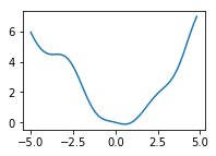
## The missing function values are filled in smoothly
## by the matplotlib-package
plt.figure(figsize = (3,2))
plt.plot(x,y)
plt.show()